Necessary considerations when estimating linkage disequilibrium at different allele frequencies

Recently, I have been going through old notes I never published. I’m going to try and post a few as blogs over the next few months. The background here is that in 2021 I was examining linkage disequilibrium (LD) for nonsynonymous and synonymous sites in microbial species using Human Microbiome Project metagenomic data. It soon became clear that one must carefully choose how LD is estimated. Below are some basic simulation results from 2021, unedited, with a minor addendum.

Notes

We are interested in estimating LD in natural microbial populations, defined as

Typically, this quantity is calculated across the joint Site Frequency Spectrum (SFS). We expect that empirical values of $\sigma_{d}^{2}$ could vary by allele frequency $f$, revealing something about selection. The plan is to bin the joint SFS and calculate $\sigma_{d}^{2}$ in each bin.

Before overinterpreting empirical estimates, it is worth considering whether the above strategy provides accurate estimates of the true LD in an ideal population with two sites, both harboring neutral mutations. We start by simulating the joint SFS of two neutral mutations at different sites with high recombination $N\cdot R \gg 1$. The SFS of a de novo mutation segregating in a population is $P(f) \sim \frac{1}{f}$. So the mutation at the second site is introduced on the same background as the mutant on the first site with probability $f$. We now have four haplotypes in the population: $f_{\mathrm{A}\mathrm{B}}, f_{\mathrm{A}\mathrm{b}}, f_{\mathrm{a}\mathrm{B}}, f_{\mathrm{a}\mathrm{b}}$. The standard coefficient of LD is $D \equiv f_{\mathrm{A}\mathrm{B}} f_{\mathrm{a}\mathrm{b}} - f_{\mathrm{A}\mathrm{b}} f_{\mathrm{a}\mathrm{B}} = f_{\mathrm{A}\mathrm{B}} - f_{\mathrm{A}} f_{\mathrm{B}} $, where $R\cdot D$ reflects the rate of change in the frequency of a haplotype due to recombination per-generation. So population sizes at the next generation are drawn as a multinomial, with the following update rules:

Basically, a Wright-Fisher model where the simulation stops if any allele goes extinct (i.e., denominator of LD = zero). We are focusing on the parameter regime $N \cdot R \gg 1$, so \(\left < \sigma_{d}^{2} \right > \approx \frac{1}{2NR}\) with $10^{6}$ simulations. Let’s look at the SFS for $f_{\mathrm{A}\mathrm{B}}$ and the marginal frequencies $f_{\mathrm{A}} and f_{\mathrm{B}}$.

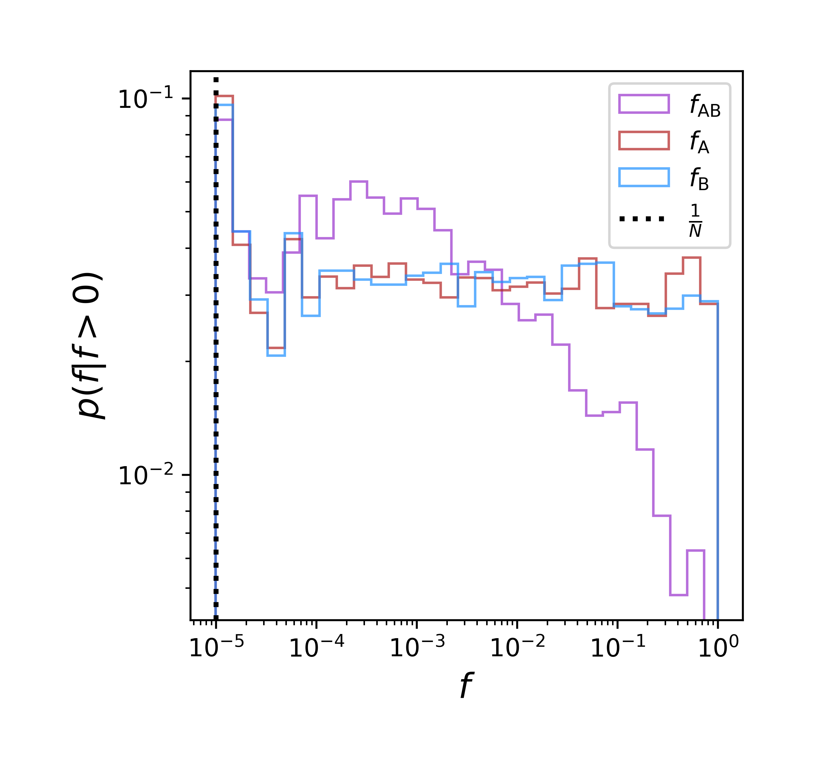
The range of the distribution of $f_{\mathrm{A}\mathrm{B}}$ is small and the distribution has a noticeably different form. LD calculated from this simulated data is close to the value predicted under quasi-linkage equilibrium (0.000534 vs. 0.0005), so our simulations appears reliable. And the different forms of the distributions used to calculate LD tell us that arbitrarily binning by frequency will introduce biases even in this easily understandable evolutionary scenario. This isn’t the whole story, however. “Frequencies” in empirical data are outcomes of sampling. We can sample our simulated data as a multinomial and estimate LD. A generous sample size of $10^{4}$ gives a mean squared error of $\sim 0.014 \% $. A more realistic sample size of $10^{2}$ gives us a MSE of $\sim 1.0 \% $. These deviations are also all biased in that they report an LD greater than its true value. Clearly sampling is an essential consideration.

What happens when we calculate LD for binned frequencies? Let’s define our binning strategy so that intervals are logarithmically spaced, as our neutral SFS is a power law. So, linear sliding windows of $\left[ \mathrm{ln} f^{\ast }, \mathrm{ln} f^{\ast }+ \Delta \mathrm{ln} f^{\ast } \right]$ (this also isn’t a critical choice). This test should be straightforward, as we are simulating a parameter regime where the LD should be constant with respect to frequency windows.

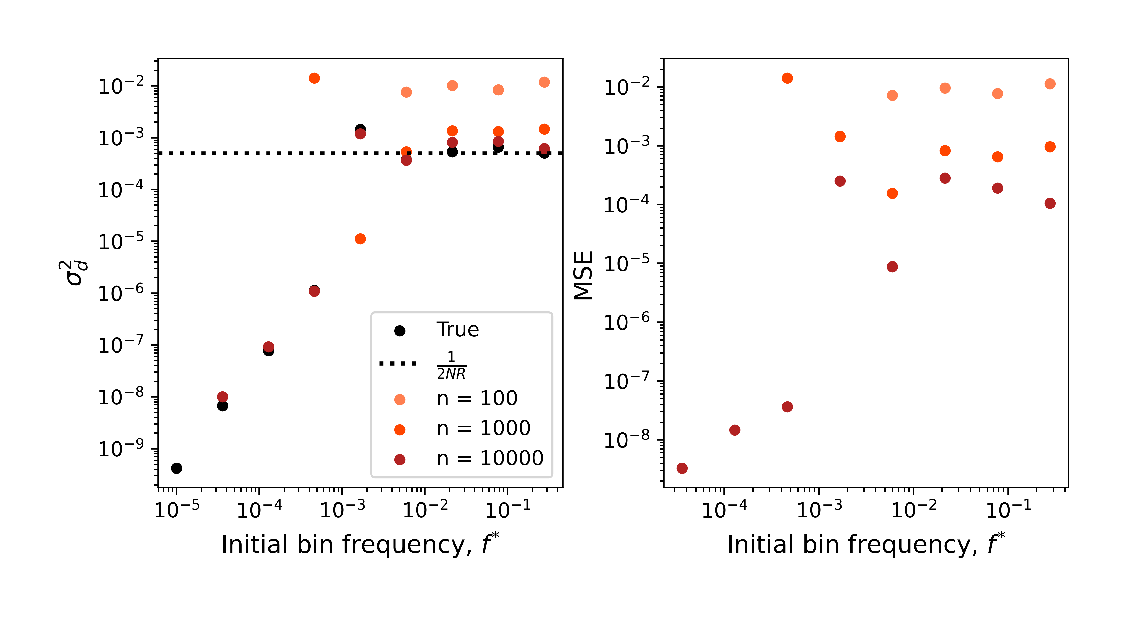
Similar deviations occur if we apply to this binned data the sample-size aware estimator developed for non-binned data (Garud, Good et al., 2020). There doesn’t seem to be a surefire way to correct this bias post hoc. A sampling-aware estimator will need to be derived for binned intervals. Recently a weighted estimator of LD has been proposed (Good, 2022). It’s worth weighing the pros of cons of binning vs. weighing if we want an interpretable estimator of LD.

Addendum

Sampling is ineluctable. This is true in general, but its consequences are especially important if your evolutionary dynamics of interest can be described as an origin-fixation process, meaning that you expect some fraction of alleles to be rare when sampled. So, it is important to consider how sampling can be integrated into your analysis. Us microbiologists are in luck, as microbial sequence data, both for ecology and evolution, often permits sampling to be modeled as a Poisson process. Also, in this years-old chickenscratch I centered interpretable simulations with minimal overhead. I still think this is crucial if you want to explain something, especially in the initial stages of a project. In practice, this means that you have to be able to point and say what does what in your model.

References

Garud, N. R., B. H. Good, et al. “Evolutionary dynamics of bacteria in the gut microbiome within and across hosts.” PLoS biology 17.1 (2019): e3000102.

Good, B. H. “Linkage disequilibrium between rare mutations.” Genetics 220.4 (2022): iyac004.